How many words do you know?
A few years back, I started wondering: what’s the minimum number of questions you’d need to ask someone to figure out the size of their vocabulary? Of course, asking random questions is not exactly optimal, and clearly the best solution would involve some kind of exploration-exploitation trade-off, but I never got around to actually work on it. Now that I’ve got some free time, I figured I’d give it a shot.
Here’s how I’ve been conceptualizing the problem: imagine having a list of all words, ranked by their difficulty. If I assign a prior probability to each of these words and begin sampling from this distribution, I can use the answers to update the prior, repeating the process iteratively. This is essentially a version of Thompson Sampling.
To develop an appropriate probability distribution for knowing a word, it’s useful to consider that people are more likely to know easier words than more difficult ones. This insight is critical, as it helps us define the structure of the distribution. I hypothesize that the distribution is shaped like an inverted sigmoid (S-curve).
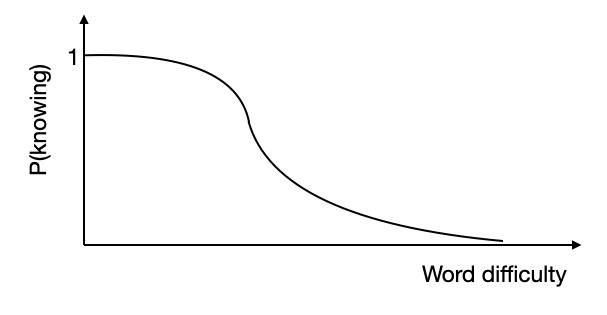
Thus, our goal is to identify this distribution by asking vocabulary questions. We assume that words, denoted by $w_i$, are ordered by their difficulty, $x_i$, which corresponds to their rank in the list. The user’s knowledge of vocabulary can be modeled as follows:
\[\begin{equation} p(w_i) = \frac{1}{1 + e^{(x_i - \mu) / \sigma}} \end{equation}\]where $\mu$ and $\sigma$ represent the mean and standard deviation of the distribution of words the user knows. This distribution can serve as the prior, from which we will sample words. The algorithm for iteratively updating the prior is as follows:
Algorithm: Iterative Prior Update
- Sample a random word, $w_i$, from the prior and ask the user if they know the word. The answer, $y_i$, is binary: {0, 1}.
- Add the data point $(x_i, y_i)$ to the dataset, $D = {(x_i, y_i)}_{i=1}^N$.
- Update the prior by fitting Equation (1) to D using maximum likelihood estimation, and calculate the new values of $\mu$ and $\sigma$.
While this is a relatively simple model, it works surprisingly well in practice.
We could also get a bit fancier, and implement a bayesian logistic regression model instead. The algorithm is basically the same, but instead of using MLE, we have to use variational inference to estimate the posterior. In practice, these two approaches behaves slightly differently, which I will mention later.
Implementation
Here is a simple implementation in Python:
Vocabulary Knowledge Quiz Using Thompson Sampling
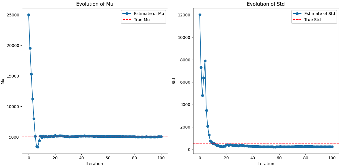
In order to see how well the algorithm works, we can simply create a user simulation with a known $\mu$ and $\sigma$, and try to iteratively find the distribution. Here is the results for the non-bayesian approach:
and the results for the bayesian approach:
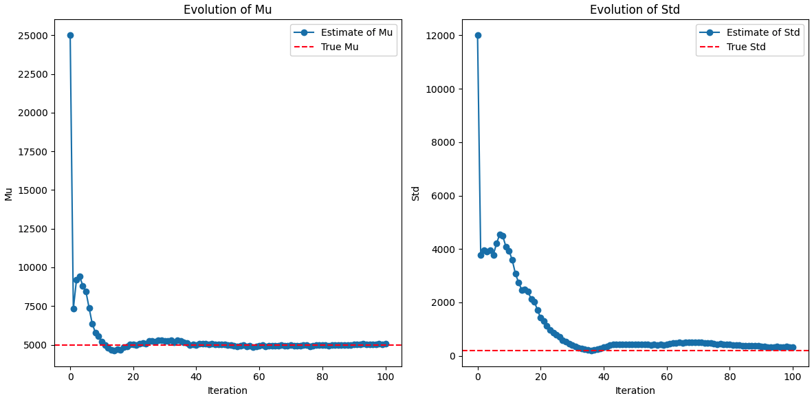
Typically, the bayesian approach overestimates the standard deviation, whereas the non-bayesian approach underestimates it.
I also implemented an actual quiz, where the user answers questions about vocabulary. The challenge with that was the fact that getting an actual list of words ordered by difficulty is not exactly simple. I assumed that word difficulty is the same as word frequency, but that is not always correct. When doing the test, I often found cases where a simpler word had a much lower frequency that a harder word. The impact of that was that with the non-bayesian approach, the algorithm was too quick to narrow down the distribution, and a few lucky draws in the beginning, changed the outcome. With the bayesian approach, the algorithm was more stable, and different runs resulted in closer estimates.
Now going back to the problem of knowing the extent of the vocabulary of someone, my experiments showed that it typically takes 10-20 questions to get close to the true vocabulary size using this approach. You can try it out for yourself, by cloning the repo, and running the vocabulary_quiz.py script.