The first time I heard about how diffusion models work, I was dumbfounded! How can you start from random noise, denoise it over and over, and get a clean generated image? In other words, how can no information result in a lot of information? There are many papers and blog posts explaining the math behind this, and honestly, it may even seem intimidating at first, but when you understand the intuition behind it, you realize how beautiful it is. So in this post, I’d like to write down my understanding and intuition about diffusion models with as little math as possible.

What is the diffusion model about?

Simply put, the goal of diffusion modeling is to sample from a high dimensional distribution without having direct access to it. But you might ask what does this have to do with image generation? Let me explain!

Imagine a 100×100 pixel (grayscale) image: we can reshape it into a vector of size 10,000. Rescale the values to be between 0 and 1. Now you can see that the space of all possible images of size 100×100 exists within a 10,000-dimensional hypercube.

Here’s the key insight: What is the distribution of all “good” photos in this space? By good, I mean meaningful, not blurry, not distorted, not noisy, etc. If we could visualize this hypercube, we’d see that it’s mostly empty, except for some lower-dimensional manifolds where good photos lie.

The proof is simple: What’s the probability of getting a good photo by randomly sampling a point from this hypercube? If you randomly generate 10,000 independent samples from [0, 1] and arrange them as pixels, how likely are you to see a meaningful image? Almost zero. This is why the space is mostly “empty”—but not completely, since every real photo exists somewhere in that space.

So we have a clear picture: the distribution of good images forms complex, unknown manifolds in high-dimensional space. We want to sample from these manifolds, but we don’t have direct access to this distribution. This is where things get interesting.

Langevin Sampling: The Foundation

The key insight comes from Langevin dynamics. If we want to sample from some distribution P(x), we can start from a random point and iteratively move toward high-probability regions using the score function (gradient of the log-probability). Think of this as gradient ascent on log-probability density, but with strategic noise injection to prevent mode collapse, and facilitate exploration.

The discretized Langevin sampling algorithm for a distribution P(x):

sample x from N(0, 1)
for t in range(T):
    sample z from N(0, 1)
    x = x + 0.5 * ε * ∇_x log P(x) + sqrt(ε) * z
return x

where ε is a step size hyperparameter, much like learning rate. Let’s address the key questions:

Why the gradient? We want higher probability of sampling from high-probability regions. The gradient points toward areas of increasing probability density.

Why gradient of log P(x)? The log transform has nice properties: where $P(x)$ is very small, $\nabla \log P(x)$ becomes large, so we move faster toward probability mass. Where $P(x)$ is large, the gradient is smaller, preventing overshooting.

Why add noise? It’s obvious that without noise, we’d converge to local modes (much like gradient ascent!). The noise term enables exploration across different modes of the distribution, giving us diverse samples rather than just point estimates.

This extends naturally to high dimensions where our image space lives. The problem remains: how do we compute $\nabla_x \log P(x)$ when we don’t know $P(x)$?

Where Denoising Comes In

Here’s the beautiful connection that makes everything work.

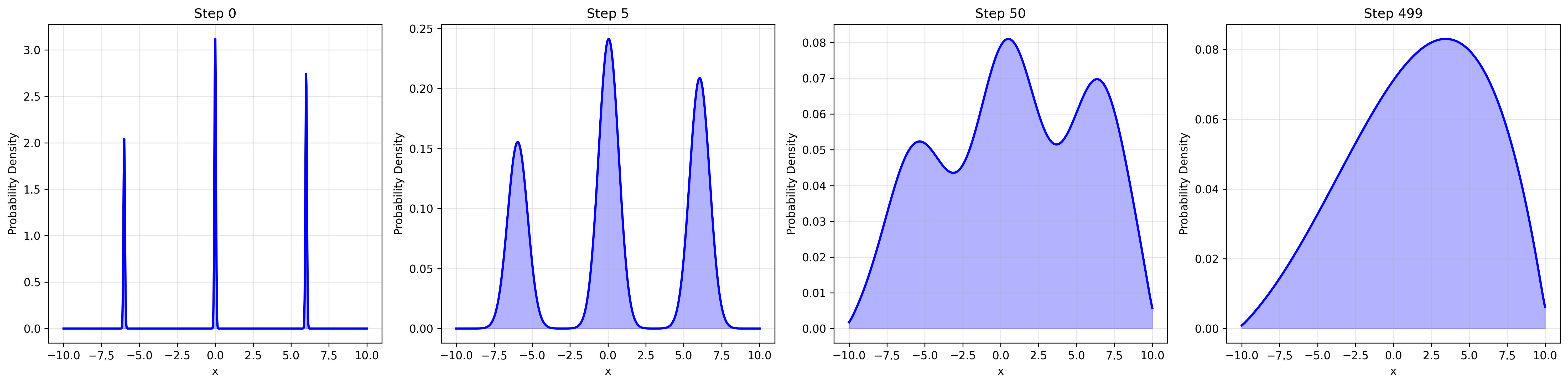
Consider what happens when we add Gaussian noise to samples from distribution $P(x)$. The distribution becomes “smoother” and spreads out. Keep adding noise, and we eventually get pure Gaussian noise. This is the forward diffusion process—we’re essentially convolving $P(x)$ with progressively larger Gaussian kernels.

Now consider the reverse: if we can go from a noisier version of the distribution to a less noisy one, we’re moving in the direction of the gradient of the log-probability!

Here’s the mathematical key. For a noisy version $x_t$ with noise level $\sigma_t$, we have:

\[\nabla_x \log p_t(x_t) = -\frac{1}{\sigma_t^2}(x_t - E[x_0 \mid x_t])\]

where $E[x_0 \mid x_t]$ is the expected clean image given the noisy observation. This is straightforward to derive from the Gaussian noise model.

But $E[x_0 \mid x_t]$ is exactly what a denoiser estimates! So:

\[\nabla_x \log p_t(x_t) \approx \frac{1}{\sigma_t^2}(\text{Denoiser}(x_t) - x_t)\]

This is the core insight: the direction a denoiser moves an image is proportional to the score function we need for sampling.

Now our sampling algorithm becomes:

sample x_T from N(0, I)
for t in range(T, 1, -1):
    sample z from N(0, 1)
    s = (1/σ_t²) * (Denoiser(x_t, t) - x_t)
    x_{t-1} = x_t + 0.5 * α_t * s + sqrt(α_t) * z
return x_0

Training the Denoiser

The training procedure is elegant in its simplicity. We don’t need to add noise step by step during training—we can jump directly to any noise level using the reparameterization trick.

For any timestep $t$, we can write: $x_t = \sqrt{\bar{\alpha}_t} x_0 + \sqrt{1 - \bar{\alpha}_t} \epsilon$

where $\bar{\alpha}_t$ comes from the noise schedule and $\epsilon \sim N(0, I)$. This closed-form allows us to create training pairs $(x_t, t)$ from any clean image $x_0$.

The training objective is simple: predict the noise $\epsilon$ that was added.

\[\text{Loss} = E[||\epsilon - \epsilon_\theta(x_t, t)||^2]\]

where $\epsilon_\theta$ is our neural network (typically a U-Net) that takes as input the noisy image $x_t$ and timestep $t$.

Why predict the noise instead of the clean image? Both formulations are mathematically equivalent, but empirically, noise prediction works better. The intuition is that the model learns to identify what doesn’t belong (the noise) rather than reconstructing what should be there.

Why condition on timestep t? Different noise levels require different denoising strategies. Light noise needs subtle corrections, while heavy noise requires more aggressive restoration. The timestep embedding allows the network to adapt its behavior accordingly.

During inference, we apply the denoiser iteratively. Even though it was trained to predict the full noise in one shot, we only use its output to make small corrections at each step. This works because we’re using the score estimate (denoising direction) rather than the full denoising result.

Summing It Up

Tying it back to our 100×100 image example: a good intuition is that after training, we implicitly know the gradient direction of P(x)—the distribution of all good images—at every point in our 10,000-dimensional hypercube. So when we pick a random point in that space, the path to a generated photo is already carved out, though it has to be done step by step (almost, since we add random noise at each step, which keeps us exploring rather than following a deterministic path). This is why we can start from what appears to be pure noise and end up with a meaningful image!

References

FAQ

Why is it called diffusion model?

The name comes from the forward process, where we gradually add noise to images until they become pure random noise. This process resembles how particles diffuse in physics—starting from a concentrated state and spreading out until they’re uniformly distributed. In our case, the “information” in a structured image diffuses away into randomness.

However, the naming is honestly a bit confusing and could be better! These models have nothing to do with the actual diffusion equation from mathematics (the partial differential equation ∂u/∂t = ∇²u). The connection is purely metaphorical. A more accurate name might be “denoising score models” or “iterative refinement models,” but “diffusion” stuck because the original papers framed the problem in terms of this forward diffusion process.

How do people use prompts to generate images?

This is where conditioning comes in, and it actually does not require much change! The core idea is to modify our denoising network to be conditioned on additional information—in this case, text embeddings.

Instead of just training ε_θ(x_t, t), we train ε_θ(x_t, t, c) where c is the conditioning information. For text prompts, c is typically created by:

Text encoding: The prompt is passed through a pre-trained language model (like CLIP’s text encoder or T5) to get a rich embedding that captures semantic meaning.
Architecture integration: This embedding is injected into the U-Net at multiple layers, often through cross-attention mechanisms. The model learns to attend to relevant parts of the text embedding when denoising different regions of the image.
Training with pairs: During training, we use (image, caption) pairs instead of just images. The model learns: “when denoising this noisy image, pay attention to this text description.”

The beautiful part is that this doesn’t change the fundamental sampling process—we still start from noise and iteratively denoise. But now at each step, the denoiser is guided by the text embedding, steering the generation toward images that match the prompt.

How to Tame Your Deep RL

Teaching (tiny) LLMs to Play Text-Based Games Using RL (on a $300 GPU)